GANs: how to separate quality, diversity and memorisation

On 10 June 2014, Ian Goodfellow and seven co-authors submitted “Generative Adversarial Nets”, the paper that formulated generative adversarial networks, or GANs. Its idea was precise rather than magical: train a generator that makes samples alongside a discriminator that tries to distinguish them from real data. That game later produced remarkably convincing images, but “looks real” has never meant “is diverse,” “does not copy,” or “faithfully represents the world.”

That is the durable capability gained from understanding a GAN: when faced with any generative-model demonstration, separate five questions that showcases tend to blend together—visual fidelity, diversity, memorisation, usefulness for a task and the cost of producing each sample—and add a sixth that architecture alone cannot settle: content provenance.

Two networks and an objective neither controls alone

The generator turns a random input, usually a noise vector, into a candidate sample. The discriminator receives real and generated samples and estimates which group each came from. During training, the discriminator learns to be right, while the generator receives a signal that helps it make examples that are harder to reject. There is no human catalogue telling it which nose, texture or edge to draw: information arrives through the adversary’s errors.

The foundational paper expresses the process as a minimax game. Under ideal assumptions—enough capacity and optimisation of the discriminator at each step—it shows that the solution has the generated distribution equal to the data distribution, with the discriminator returning 1/2 everywhere. That is a mathematical property of the ideal model, not a certificate that two finite networks trained on a limited number of images have reached it. In practice, approximate updates alternate, and a modified generator loss is used to avoid excessively weak gradients early in training.

The gap between objective and procedure matters. If the discriminator learns much faster, it may reject almost everything without giving the generator a useful direction. If the two change at incompatible rates, learning can oscillate. And if the generator finds a small set of outputs that fool its rival, it may repeat them while abandoning entire regions of the data. This failure is called mode collapse: high local plausibility, low global coverage.

What each milestone changed—and what it did not solve

In 2015, DCGAN combined architectural choices—strided convolutions, batch normalisation, removal of certain fully connected layers and particular activations—and demonstrated useful visual representations. It did not prove that adding convolutions stabilises every GAN; it documented a family of constraints that worked in its experiments.

In 2017, Wasserstein GAN replaced ordinary discriminator classification with a critic and an objective with better properties for tracking training progress. The paper sought more meaningful learning curves and less mode collapse. It did not make training automatically reliable: the critic must satisfy constraints, and later work proposed other ways to enforce them.

The applications also teach readers how to interpret limits. CycleGAN learned mappings between two domains without paired examples by using cycle consistency. It can turn horses into zebras or change seasons in a scene, but the mapping is not determined by observed pixel-for-pixel truth; a plausible output can introduce features that were never in the input. SRGAN optimised perceptual super-resolution and produced textures that looked more convincing than solutions aimed only at squared error. That does not necessarily recover the lost original detail: it proposes detail compatible with what the system learned.

The same caution applies to modern restorers such as Real-ESRGAN, which constructs synthetic degradations to better approach real photographs. A restored image can be useful and attractive without becoming forensic evidence of what the sensor captured. The more a task depends on exactness—medicine, documents or evidence—the less adequate it is to ask only whether the output looks good.

Quality and coverage are not the same measurement

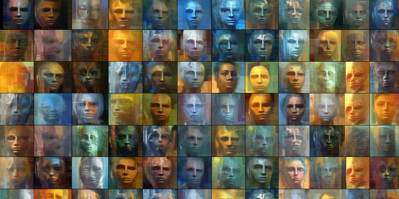
A grid of twenty spectacular samples answers only one question: the system can produce at least those examples. It does not reveal how many attempts were discarded, whether it repeats variants of the same faces or whether it remembers training images. Serious evaluation needs a test set and a reproducible protocol.

The 2017 work that introduced the Fréchet Inception Distance (FID) compares feature statistics extracted from real and generated images. A lower FID can be informative when models, data, preprocessing and sample counts are comparable. It is not a universal realism score: it summarises distributions through a particular approximation, depends on the feature extractor and protocol, and does not justify comparisons between figures calculated through different pipelines.

Another NeurIPS paper explicitly separated precision and coverage for generative models. In this reading, precision asks what proportion of generated samples lies near the real distribution: it approximates fidelity. Coverage, or recall, asks how much of the real space the generator reaches: it approximates diversity. A model can improve one while sacrificing the other. “Our output is more realistic” is therefore incomplete without the metric, dataset, sample count, reference and range of variation.

Memorisation requires a different test. Evaluators should look for close neighbours of outputs in the training set, repeat the analysis on unseen data and check whether some groups appear disproportionately often. For an application, the decisive test may be different again: measure whether synthetic data improve a downstream task evaluated on held-out real data. No curated screenshot can replace those checks.

Diffusion does not mean universal replacement

The denoising diffusion probabilistic models presented in 2020 learned to reverse a gradual noising process. In 2021, “Diffusion Models Beat GANs on Image Synthesis” showed that an improved version achieved competitive or superior results on specified image benchmarks and examined the trade-off between quality and diversity. It was an experimental comparison under defined configurations and metrics, not a law retiring every GAN.

The operational distinction helps with selection. After training, a GAN normally generates through one pass of the generator; classical diffusion performs a sequence of denoising steps, although research has reduced that number. This latency can favour GANs in video, restoration or interactive systems. Diffusion has become prominent for broad-purpose image generation, while GANs remain an option where speed, domain translation or a specialised design carries more weight. “Which family wins?” has no answer without a task, hardware, required quality and inference budget.

A checklist for reading the next demonstration

First, identify the comparison data: dataset, resolution, preprocessing, number of samples and baseline. Second, separate fidelity from diversity; one score or a gallery does not cover both. Third, look for a memorisation test and results by subgroup, not just an average. Fourth, demand evaluation on unseen real data when practical usefulness is promised. Fifth, compare time, memory and energy per sample on the same hardware. Sixth, ask where the data came from and how synthetic output will be identified.

The final point prevents a fundamental confusion: a GAN’s discriminator is a training component, not a universal authenticity verifier. An output fooling that rival does not prove that it came from a camera, or that it will fool every person or future detector. Perceptual quality, documentary truth and provenance are different problems.

The lesson from 2014 remains alive precisely because it supports this sober reading. The adversarial game introduced a powerful way to approximate complex distributions, and its failures taught the field not to mistake a brilliant sample for a complete model. Faced with the next “indistinguishable from reality,” the competent response is neither belief nor denial. It is to ask: indistinguishable to whom, measured how, with what coverage, against which data and at what cost?