Time Series

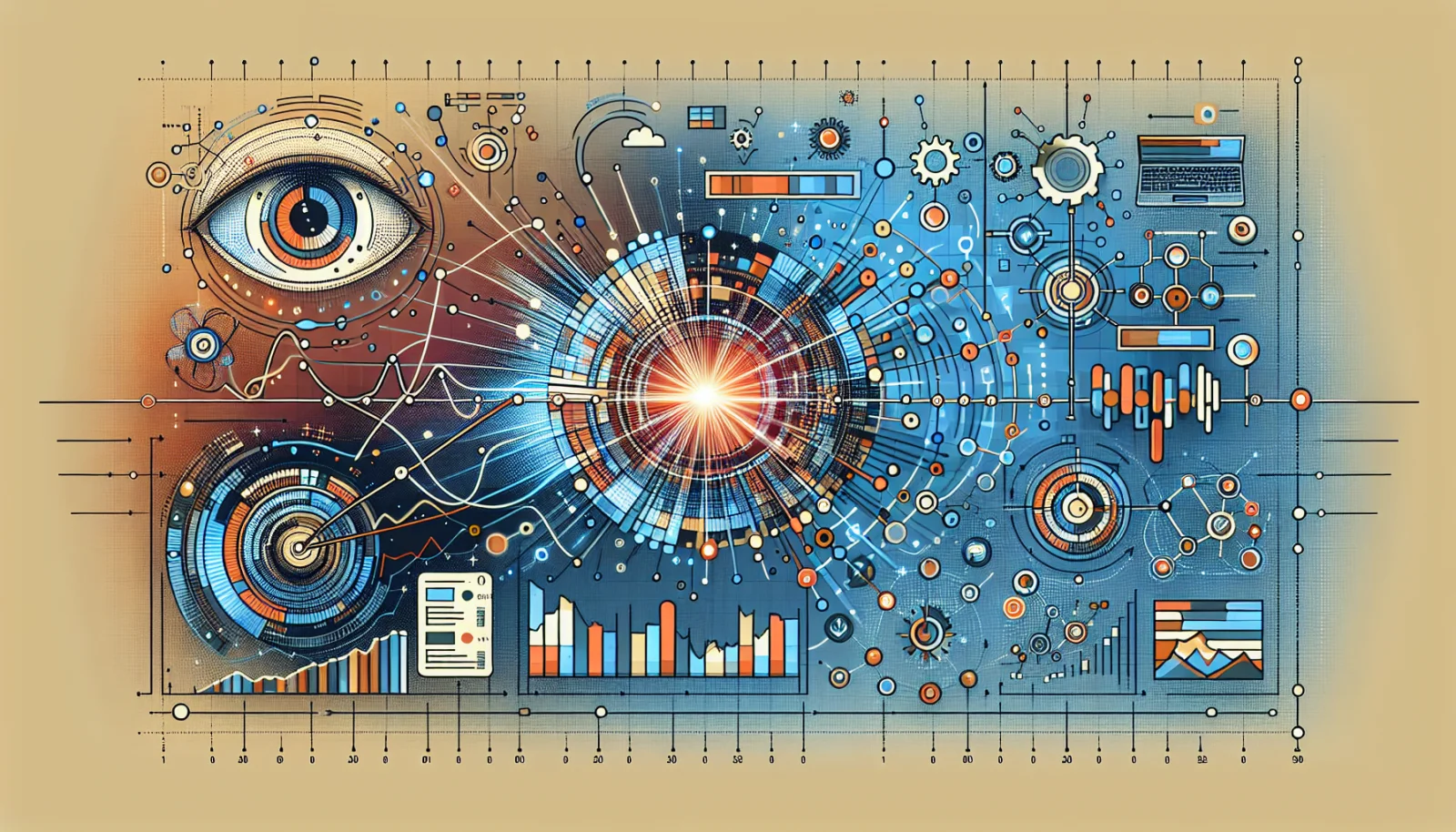
A time series is a sequence of observations ordered in time, most often recorded at regular intervals: a stock's daily price, hourly temperature, a city's electricity demand, or the periodic reading of a sensor. What sets it apart from any other dataset is that order matters: each value is related to the ones before it, and shuffling the observations destroys that information.

The most common task is prediction, or forecasting: anticipating future values from past ones. Time series are also used to flag anomalies, monitor a process, or pull patterns apart. When the observations are spread across space as well —sensor networks, satellite imagery— the problem moves into spatio-temporal analysis, which has its own entry in this glossary.

Trend, seasonality, and noise

A series is usually read as the sum of three components. The trend is the long-run direction, such as demand that grows year after year. Seasonality is the set of patterns that repeat over a fixed period: more electricity in winter, more web traffic on Mondays. The noise, or residual, is what remains once the first two are removed, the irregular part no model should try to memorize. Pulling these pieces apart is called decomposition, and the standard reference by Hyndman and Athanasopoulos, «Forecasting: Principles and Practice», treats it as a step that precedes any serious model.

Stationarity and autocorrelation

Many classical methods require the series to be stationary: its statistical properties, such as the mean and variance, must not change over time. A series with a trend or with seasonality is not stationary, but it can often be made so by differencing, that is, subtracting each value from the one before it. The other central idea is autocorrelation: the correlation of the series with a lagged copy of itself. It measures how much memory the process carries, and in practice the way the autocorrelation function (ACF) decays reveals whether a series is stationary and which model might suit it.

From ARIMA to neural methods

The classical toolkit begins with George Box and Gwilym Jenkins, whose 1970 book popularized ARIMA models (autoregressive, integrated, moving average) and a three-stage method: identify, estimate, and diagnose. Alongside them sit exponential smoothing (Holt-Winters) and state-space models. Since the 2010s, neural methods have gained ground: recurrent networks and LSTMs to capture long dependencies, and newer architectures such as N-BEATS (Oreshkin and colleagues) or Transformers adapted to sequences. In parallel, tools like Prophet, released by Facebook in 2017, put forecasting within reach of analysts without deep statistical training. No method wins every time: over short horizons and clean series, ARIMA remains hard to beat.

Validating without temporal leakage

Evaluating a time-series model has one non-negotiable rule: respect the order of time. Ordinary cross-validation shuffles the data at random, and on a series that means training on the future to predict the past, a temporal leak that inflates the metrics and misleads. The correct approach is forward validation (walk-forward, or backtesting): train only on the past and always test on the stretch that follows, as scikit-learn's TimeSeriesSplit does. The open questions start here: on non-stationary series or those with structural breaks, no validation scheme guarantees that measured performance will hold, and whether large neural models consistently beat the classics remains an open debate.