GNSS super-resolution: what improved by 62%—and what it did not forecast

On August 14, 2025, a team including researchers from Wrocław University of Environmental and Life Sciences published a method for refining GNSS-derived tropospheric tomography. A generative network converted low-resolution three-dimensional fields into finer estimates of wet refractivity and outperformed both the original tomography and conventional interpolation in two case studies, Poland and California.

That does not yet mean flood warnings became 62% better. The original scientific article measures reconstruction error against Weather Research and Forecasting model outputs and radiosondes. The durable skill is understanding what scientific super-resolution promises: it does not observe new details by magic. It estimates likely structures from coarse data and learned patterns, and must show that those structures agree with independent observations.

GNSS does not directly photograph humidity

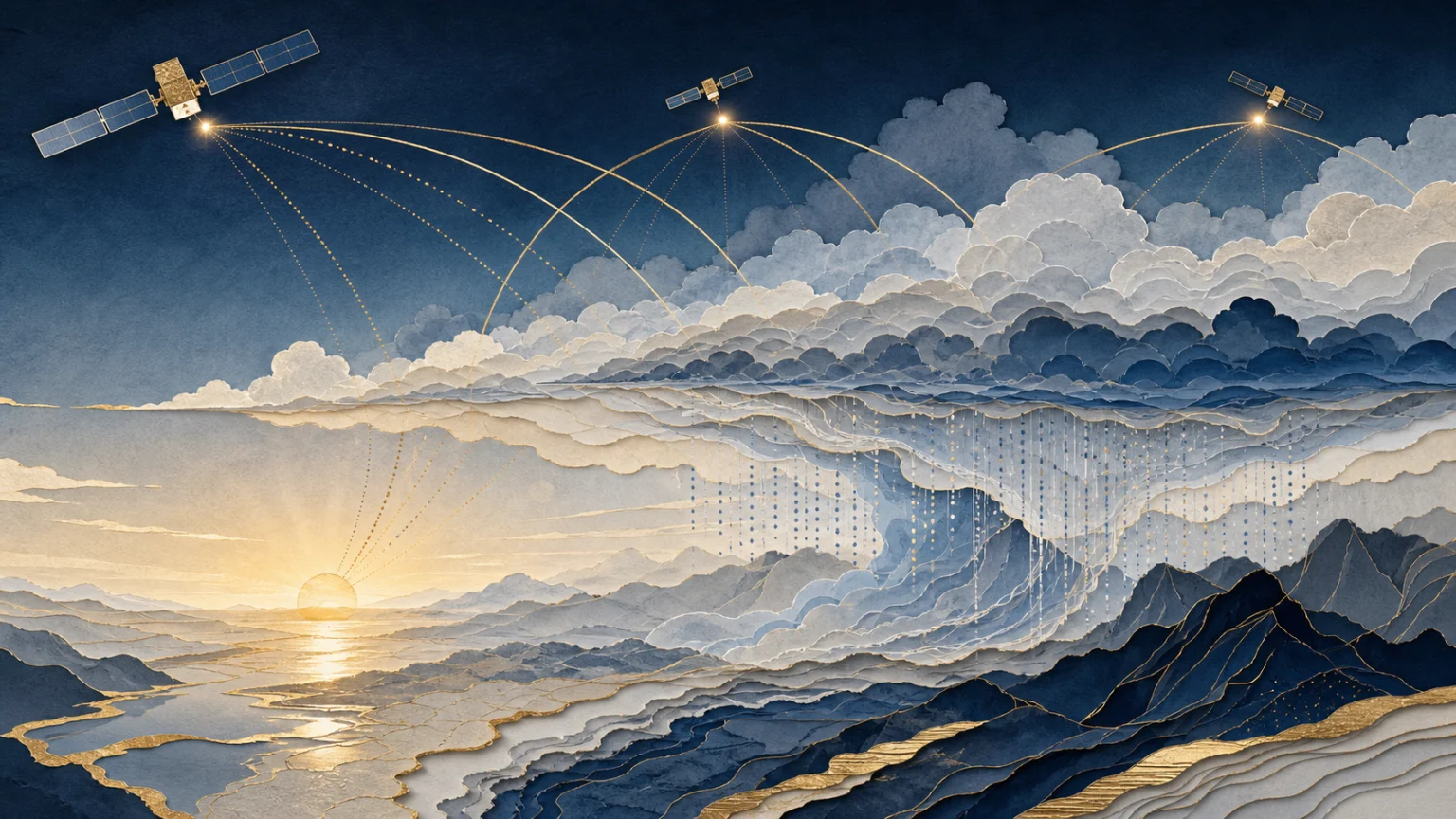
GPS, Galileo and other GNSS satellites transmit radio signals for positioning. As those signals cross the troposphere, they are delayed. Part of the delay is associated with dry gases and another part with atmospheric water. Ground stations, satellite geometry and models can estimate delays along many paths.

Tomography divides the atmosphere into voxels and attempts to reconstruct wet refractivity in each cell. The inverse problem is ill-conditioned: there are more unknowns than observations, and many voxels are not crossed by a useful ray. The solution needs regularization or external information. It is therefore not a direct reading of every cube of air.

The study’s central variable is wet refractivity, measured in parts per million. It is related to water vapor and temperature, but calling it simply “humidity” removes a physical step. The map is not a vapor camera; it is a reconstruction of how the wet component of the atmosphere affects signal propagation.

The open-access paper PDF also explains that hydrostatic delay was calculated with WRF surface-pressure output and that the Poland and California inverse problems used different solution methods. The input product already combines measurements, geometry, assumptions and modeling.

What the network adds—and where detail comes from

The team used an SRGAN, a super-resolution generative adversarial network. Its generator receives coarse maps and produces fine ones; its discriminator learns to distinguish generated outputs from reference fields. Content and adversarial losses push the result toward the high-resolution patterns seen in training.

The detailed reference came from the Weather Research and Forecasting model. The official WRF documentation describes it as an atmospheric system for research and numerical weather prediction with multiple physics options. The authors configured WRF differently for each region and used inner domains of 4 × 4 kilometers in Poland and 5 × 5 in California, at hourly resolution.

This clarifies what “increasing resolution” means. The network learns the relationship between coarse tomography and detailed WRF fields. It does not uncover texture secretly stored in every pixel. It infers the detail that usually corresponds to an input pattern according to examples. When that relationship changes, it can produce a plausible but false field—the scientific equivalent of invented sharpness in a photograph.

The method itself includes a revealing filter. Before training, the researchers excluded image pairs whose correlation between tomography and WRF was below 0.4. About 97% of the remaining data went to training and validation, and 3% to testing. The filter makes a coherent relationship easier to learn, but bounds applicability: cases where input and reference strongly disagree are not the ground on which success was measured.

That distinction matters in any scientific enhancement system. A model can score well because it handles representative cases, because the benchmark excludes difficult mismatches, or because train and test samples share weather regimes that recur in time. Those explanations demand different confidence. A strong evaluation therefore reports not only an aggregate score, but the sampling dates, geographical separation, exclusion rules and performance on rare conditions. Readers should look for that audit trail before treating a sharper grid as a more truthful one.

What 62% and 52% mean

The two numbers are maximum relative reductions in root mean square error, not universal averages. In Poland, 62.2% occurred above 6,000 meters when WRF was the validation reference; against radiosondes, the reduction in that band was 26.1%. In California, 52% occurred from 3,000 to 6,000 meters against WRF; against radiosondes, it was 32.8%.

Other altitudes improved by other amounts. Below 3,000 meters, Poland showed reductions of 41.67% against WRF and 26.51% against radiosondes. California achieved 45.29% and 35.43%, respectively. “Reduced error by 62% in Poland” is accurate only if it retains “up to” and identifies altitude and reference.

The authors warn that wet refractivity above 6,000 meters is often very small, near zero. A small absolute difference can yield a large relative RMSE change without much practical significance. That note changes the interpretation of the most attractive figure: the largest percentage need not mark the most important meteorological benefit.

Nor are these “forecast errors.” They are errors in the downscaled product relative to references. Showing better warnings would require assimilating the fields into a forecasting system, running forecasts with and without them, and measuring rain, location, lead time, false alarms and missed events. The study proposes that future use; it does not report that operational trial.

Two references are better than one, but not equivalent

WRF supplies a continuous high-resolution field, ideal for cell-by-cell comparison. It is nevertheless another model, not the atmosphere itself. If the SRGAN learns to imitate its biases, strong agreement with WRF can overstate progress. That is why additional validation against radiosondes matters.

A radiosonde is a balloon-borne sensor package transmitting pressure, temperature, relative humidity and position. The US National Weather Service describes radiosondes as a primary source of upper-air observations and ground truth for satellite data. They provide a physical measurement, but only along specific paths and times; they do not cover every voxel.

Performance against both references is more persuasive than performance against WRF alone. Generalization still requires holding out locations, years and events so the test set is genuinely new. A “carefully selected” 3% test set spans varied conditions, but it is not equivalent to continuous prospective validation in other GNSS networks and climates.

Showing where a model looked does not show it was right

The researchers used Grad-CAM and SHAP to visualize influential regions. In Poland, attributions aligned with high refractivity and active fronts; in California, they highlighted mountainous areas and gradients. The university institute’s notice summarizes those findings and identifies validation with radiosondes and rain labeling through GPM IMERG.

An attribution answers “which parts of this input influenced this output” under a particular method. It does not establish atmospheric causality, freedom from bias or out-of-sample reliability. A model can attend to a meteorologically sensible region and still get the intensity wrong. Explainable AI is a diagnostic instrument, not a certificate.

A path to adoption contains four separate rungs: a more faithful reconstruction; a better initial condition for a forecast model; a measurable forecast improvement; and an operationally useful alert. This paper supplies strong evidence for the first and a route toward the second. The final two remain to be tested.

Scientific super-resolution deserves attention precisely when it preserves that chain of evidence. For the next headline, ask: what variable was reconstructed, where did the fine target come from, which cases were excluded, what was the validation reference and which operational outcome was measured? If those five doors are open, sharpness is evidence. If not, it may be only a convincing picture of what the model expected to see.